Optimizing Large Matrix-Vector Multiplications

The aim of this article is to show how to efficiently calculate and optimize matrix-vector multiplications y = A * x for large matrices A with 4 byte single floating point numbers and 8 byte doubles. Large matrices means that the size of the matrizes are larger than the processor cache.
Before you start reading the article you should notice the following.

• The compiler I used was gcc version 3. The newer compiler versions can optimize a lot better. So some optimization might not be necessary anymore.
• The optimizations presented here are partly processor specific. I used an AMD64 3800+ Dual Core processors. Some new processors don't need the prefetching implementation because they have already a very good internal prefetching. In some processor generations it is even counterproductive.
• Note that I used matrices with a size of multiples of 8 to simplify the code.
• The matrix-vector multiplication of large matrices is completly limited by the memory bandwidth. One core can use the full bandwidth. So vector extensions like using SSE or AVX are usually not necessary. It is interesting that matrix-matrix-multiplications don't have these kind of problems with memory bandwitdh. Companys like Intel or AMD typically usually show benchmarks of matrix-matrix multiplications and they show how nice they scale on 8 or more cores, but they never show matrix-vector multiplications.
• This code is not meant for productivity. To stay on the safe side use libraries like BLAS and LAPACK for the specific architectures.

After you have read the remarks you can go on read the article.
First of all the matrix is defined as an array of size n*n which can be accessed by A[i][j]. The index of the column is j. The row index is i. The vectors x and y are defined as arrays accessed by x[i] and y[i]. The matrix A and vector x are set to simple values. The vector y is set to zero.
The building, initialization, destroying of the arrays are defined in the functions Init and Destroy.

---

Init and Destroy

template<class T>
void Init(T** &A, T* &x, T* &y, int size)
{

	T *p;
	A = new T*[size];

	p = new T[size*size];
	for(int i=0; i<size; i++) A[i] = &p[i*size];

	x = new T[size];
	y = new T[size];

	for(int j=0; j<size; j++)
	for(int i=0; i<size; i++)
	{
		A[i][j] = 0.234;
	}

	for(int i=0; i<size; i++)
	{
		x[i] = 1.234;
		y[i] = 0;
	}
	
	
}

template<class T>
void Destroy(T** &A, T* &x, T* &y)
{

	delete[] &A[0][0];
	delete[] y;

	delete[] x;

}

---

The classic implementation of the matrix vector multiplication is

---

classic1

template<class T>

uint64_t classic1(int size, int num)
{
	
	T **A, *x, *y;

	Init(A, x, y, size);

   	uint64_t time1 = rdtsc(); 

	for(int k=0; k<num; k++)
	{

		
		for(int i=0; i<size; i++)
		{

			y[i] = 0;
			for(int j=0; j<size; j++)
				y[i] += A[i][j]*x[j];
		}	
		
	}

   	uint64_t time2 = rdtsc(); 

	Finish(A, x, y);

	
	return (time2-time1);
}

---

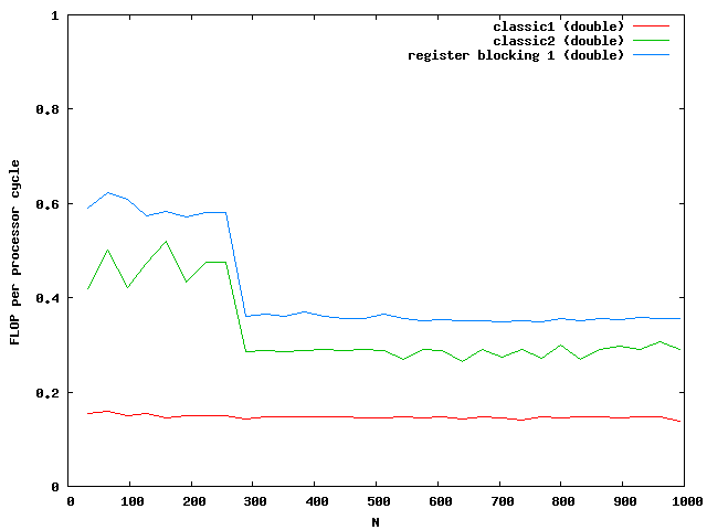
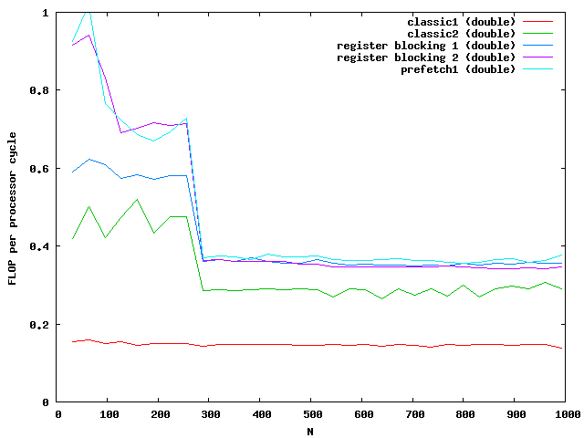
The matrix is muliplied by using the index [i][j] accessing the matrix and vector. The matrix is evaluated num times to get better results while examining the performance. The timings dependent on the size are plotted in the next picture.

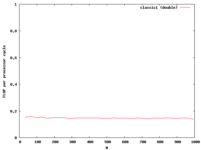
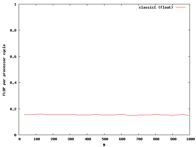
The y-axis shows the number of floating point operations per processor cycle. The test was done on an AMD64 3800+ Dual Core with 64KB First Level Cache and 512KB Second Level Cache The frequency is 2GHz , that means 2 000 000 000 processor cycles per second. The program was compiled under WindowsXP using the cygwin environment compiled with gcc 3.3 with full optimizations. The matrix is computed by around 0.18 scalar multiplications and additions per cycle. The algorithm is mainly the same for floats and doubles.

The next optimization step simply avoids accessing the matrix and vectors by indices . The computer have to read the memory in consecutive order from memory. The compiler should reckonize it and optimize it but this compiler dont. So lets see how the source code looks:

---

classic2

		T ytemp;
		T *Apos = &A[0][0];

		for(int i=0; i<size; i++)
		{

			T *xpos = &x[0];
			ytemp=0;

			for(int j=0; j<size; j++)
			{

				ytemp += (*Apos++) * (*xpos++);
			}
			y[i] = ytemp;
		}	

---

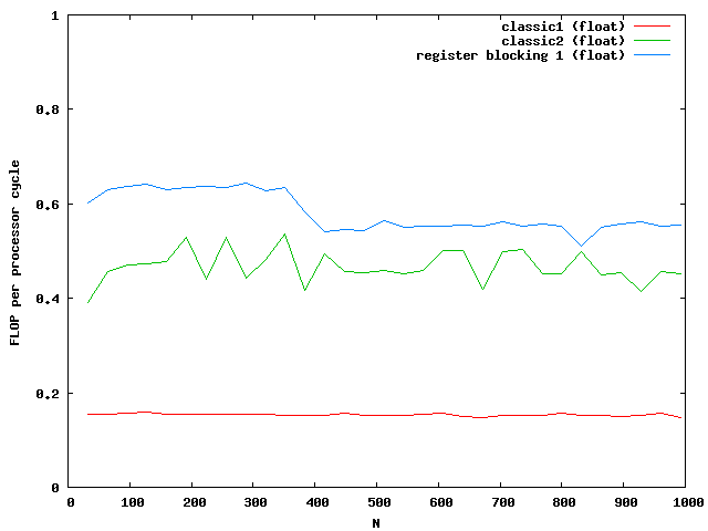
The indices are only used outside the most used loop j. The access to elements in the matrix are done via memory pointers. The speed improvement is over a factor of 2.

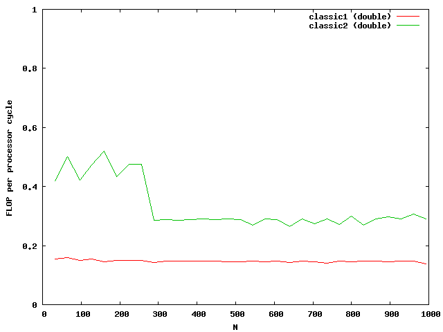
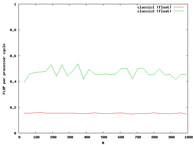
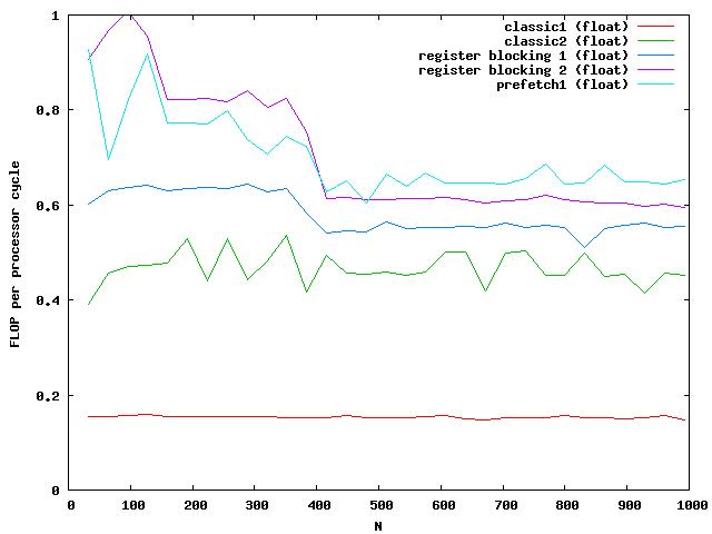
At around N=256 the size of the matrix is beyond the size of the Level 2 cache which is exactly N*N*8 = 512kB. So the memory access reduces the possible speed of the algorithm. Single floats needs half the memory and seems to be small enough that no difference between cache access and memory access are visible.
Lets look at the assembler code of the innermost loop for doubles.

loop:
fld     qword ptr [edx]
add     edx, 8
fmul    qword ptr [ecx]
add     ecx, 8
dec     eax
faddp   st(1), st
jnz     short loop

and for floats

loop:
fld     dword ptr [edx]
add     edx, 4
fmul    dword ptr [ecx]
add     ecx, 4
dec     eax
faddp   st(1), st
jnz     short loop

It looks very optimal. The memory accesses are reduced to the absolutely necessary. The solution of each row multiplication is saved in the register st(1). For out of order processor architectures it is better to mix floating point and integer arithmetics so that the processor can parallelize it. The reason is simple: the executing units for integers and floating point number are independent from each other.
We can further reduce the memory bandwidth used. The full vector x is needed in every inner loop. So lets multiply two rows in one loop.

---

register blocking 1

		T *Apos1 = &A[0][0];

		T *Apos2 = &A[1][0];
		T *ypos = &y[0];
		
		for(int i=0; i<size/2; i++)
		{

			T ytemp1 = 0;
			T ytemp2 = 0;
			T *xpos = &x[0];

			for(int j=0; j<size; j++)
			{

				ytemp1 += (*Apos1++) * (*xpos);
				ytemp2 += (*Apos2++) * (*xpos);

				xpos++;
			}
			*ypos = ytemp1;
			ypos++;
			*ypos = ytemp2;

			ypos++;
			
			// skip next row
			Apos1 += size;
			Apos2 += size;
		}	

---

The performance is

For doubles the multiplication is three times faster than the classic implementation. The floats are almost not influenced by the cache. Note that the critical size here is N = 362.
Lets do some more parallelism:

---

register blocking 2

	T *Apos1 = &A[0][0];

		T *Apos2 = &A[1][0];
		T *Apos3 = &A[2][0];

		T *Apos4 = &A[3][0];
		T *ypos = &y[0];

		
		for(int i=0; i<size/4; i++)
		{

			T ytemp1 = 0;
			T ytemp2 = 0;
			T ytemp3 = 0;

			T ytemp4 = 0;
			T *xpos = &x[0];

			for(int j=0; j<size; j++)
			{

				ytemp1 += (*Apos1++) * (*xpos);
				ytemp2 += (*Apos2++) * (*xpos);

				ytemp3 += (*Apos3++) * (*xpos);
				ytemp4 += (*Apos4++) * (*xpos);

				xpos++;
			}
			*ypos = ytemp1;
			ypos++;
			*ypos = ytemp2;

			ypos++;
			*ypos = ytemp3;
			ypos++;
			*ypos = ytemp4;

			ypos++;
			
			// skip next row
			Apos1 += 3*size;
			Apos2 += 3*size;

			Apos3 += 3*size;
			Apos4 += 3*size;
		}	

---

---

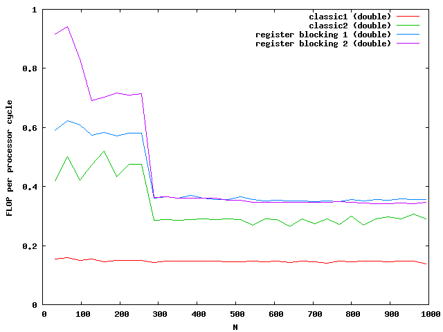
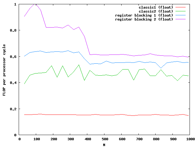
Again the speed increases for floats but not for double for large matrices. The green and purple line are on top of each other. It seems that a further increase makes no sense.
The critical sizes for level cache 1 are N = 128 for floats and N = 90 for doubles. This explains again the two slopes at the beginning.
An interesting case is a resorting of the matrix so that only one Apos is needed and this is added four times a loop. So instead of accessing four rows simultaneously one could only access one row. Tests show that this is much slower than using four rows.
This opens the question if the prefetching of the values is really optimal. Is the memory bandwidth used optimal? So as the question implies it is not. But to figure it out we have to do first some loop unrolling.

---

Prefetching 1

			register T ytemp1 = 0;

			register T ytemp2 = 0;
			register T *xpos = &x[0];

			int blocksize = size / 8;

			x0 = xpos[0];

			x1 = xpos[1];
			
			for(int j=0; j<blocksize; j++)
			{

				ytemp1 += x0 * (Apos1[0]);
				ytemp2 += x0 * (Apos2[0]);

				x0 = xpos[2];
				ytemp1 += x1 * (Apos1[1]);
				ytemp2 += x1 * (Apos2[1]);
				x1 = xpos[3];

				ytemp1 += x0 * (Apos1[2]);
				ytemp2 += x0 * (Apos2[2]);

				x0 = xpos[4];
				ytemp1 += x1 * (Apos1[3]);
				ytemp2 += x1 * (Apos2[3]);
				x1 = xpos[5];

				ytemp1 += x0 * (Apos1[4]);
				ytemp2 += x0 * (Apos2[4]);

				x0 = xpos[6];
				ytemp1 += x1 * (Apos1[5]);
				ytemp2 += x1 * (Apos2[5]);
				x1 = xpos[7];

				xpos+=8;
				ytemp1 += x0 * (Apos1[6]);
				ytemp2 += x0 * (Apos2[6]);
				x0 = xpos[0];

				ytemp1 += x1 * (Apos1[7]);
				Apos1+=8;

				ytemp2 += x1 * (Apos2[7]);
				x1 = xpos[1];

				Apos2+=8;

				
			}
			
			ypos[0] = ytemp1;
			ypos[1] = ytemp2;

			ypos+=2;
			
			// skip next row
			Apos1 += size;
			Apos2 += size;

---

In this code several additional optimizations are used. First the processor can easier predict the behavior of the following commands because there are no conidtional jumps.
Second we us here again indices but this time static. That means absolute addresses. Therefore the processor can better prefetch the values. But only if the processor supports these directly. Look at the assembler code below.

---

Prefetching 1 assembler code


loop:
fld     qword ptr [eax]
inc     esi
fmul    st, st(4)
faddp   st(1), st
fxch    st(3)
fmul    qword ptr [edx]
faddp   st(1), st
fld     qword ptr [ecx-38h]
fld     qword ptr [eax+8]
fmul    st, st(3)
faddp   st(4), st
fxch    st(2)
fmul    qword ptr [edx+8]
faddp   st(1), st
fld     qword ptr [ecx-30h]
fld     qword ptr [eax+10h]
fmul    st, st(3)
faddp   st(4), st
fxch    st(2)
fmul    qword ptr [edx+10h]
faddp   st(1), st
fld     qword ptr [ecx-28h]
fld     qword ptr [eax+18h]
fmul    st, st(3)
faddp   st(4), st
fxch    st(2)
fmul    qword ptr [edx+18h]
faddp   st(1), st
fld     qword ptr [ecx-20h]
fld     qword ptr [eax+20h]
fmul    st, st(3)
faddp   st(4), st
fxch    st(2)
fmul    qword ptr [edx+20h]
faddp   st(1), st
fld     qword ptr [ecx-18h]
fld     qword ptr [eax+28h]
fmul    st, st(3)
faddp   st(4), st
fxch    st(2)
fmul    qword ptr [edx+28h]
faddp   st(1), st
fld     qword ptr [ecx-10h]
fld     qword ptr [eax+30h]
fmul    st, st(3)
faddp   st(4), st
fxch    st(2)
fmul    qword ptr [edx+30h]
faddp   st(1), st
fld     qword ptr [ecx-8]
fld     qword ptr [eax+38h]
add     eax, 40h
fmul    st, st(3)
faddp   st(4), st
fxch    st(2)
fmul    qword ptr [edx+38h]
add     edx, 40h
faddp   st(1), st
fld     qword ptr [ecx]
add     ecx, 40h
cmp     edi, esi
jnz     loop

---

The processor loads the values independent from the values before like

	fld     qword ptr [eax+18h]

The third advantage is the better independence of the operations. Due to the using of x0 and x1 one register can be loaded while multiplicate with the other. Unfortunately the performance shows only a small increase in speed:

---

---

For the optimization step we have to go to the assembly level. For us important is especially the prefetching commands of modern processors especially the

	prefetchnta

command. This instruction loads content from memory for one time use, which is what we need for the matrix multiplication because every value is only used once. So we define

#define prefetch(mem) \
         __asm__ __volatile__ ("prefetchnta %0" : : "m" (*((char *)(mem))))

and using this at the beginning of the loop

	prefetch(Apos1+prefetch);
	prefetch(Apos2+prefetch);

Whats the best value for prefetch? Well lets see:

---

---

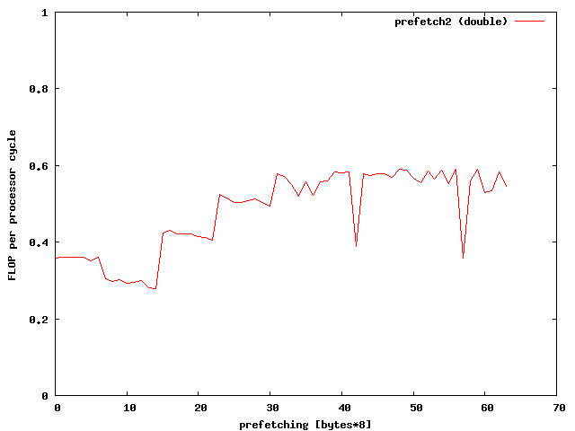
A prefetching of 32*8 bytes seems to be the right choice for doubles.

---

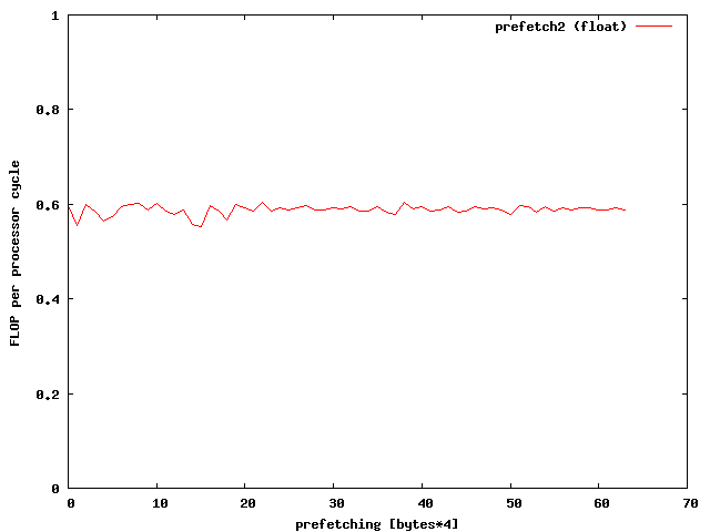
The prefetch value of 32 gives this result

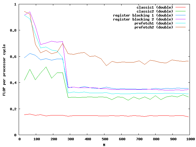
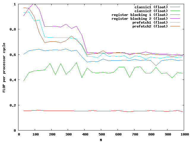
Whooww, this gives a great speed improvment. According to the memory specifications I have reached the limits of memory bandwidth for doubles. Therefore additional optimizations make no sense. To further optimize the speed for floats one might need the vectorization units like SSE or AVX of modern PCs.